Contents
Phase and angle Modulation Comparison
Effect of Frequency multiplication on the modulated signal
Effect of frequency multiplication of the modulating signal on the modulated signal
Bandwidth using Schwartz Curve
Bessel function of order n and first kind
Transmission of bitstreams using M-ary multilevel waveforms
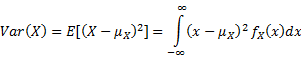
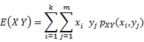
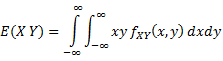
Statistical Properties of Random Variables
Binary Baseband Signal Detection
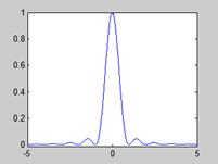
Autocorrelation & Power Spectral Density
Noise in Communication Systems
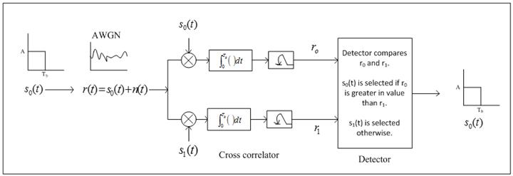
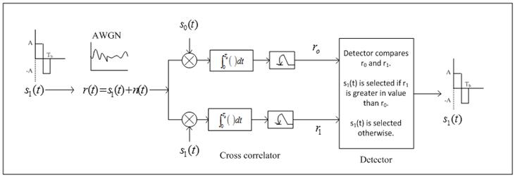
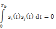
Base-band signal transmission receiver containing cross-correlator.
Probability of error calculation is the same as that of receivers with correlator
BBS through Band-limited Channels
Communication channel is a Filter
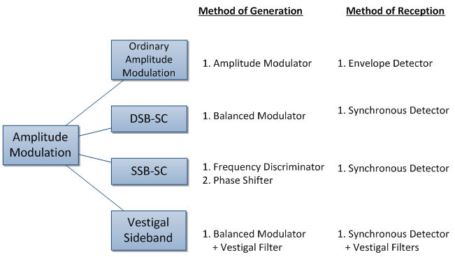
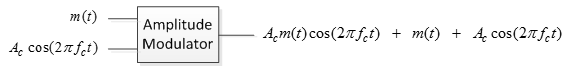
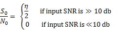
1. Conventional AM
·
![]()
·
![]() ,which means
,which means ![]()
·
![]() is the index of
modulation
is the index of
modulation
· Bandwidth=2W
·
W is the bandwidth of ![]()
·
Power in the modulated signal = ![]()
{ This relation is applicable when the modulating signal x(t) is zero-mean }
·
Total Power : ![]()
·
Current Relation : ![]()
·
Modulation Efficiency = ![]()
·
SNRO =![]()
·
Percentage Modulation(%) = ![]()
{ This relation is applicable when the modulation is symmetrical }
· Amplitude Modulator for generation.
2. DSB-AM
·
![]()
· Bandwidth= 2W
·
Power in the modulated signal = ![]()
·
SNRO = ![]()
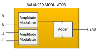
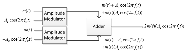
· Balanced Modulator for generation
3. SSB-AM
· ![]()
· Bandwidth = W
· Power
in the signal = ![]()
· SNRO
![]()
· Methods of generation
- Using balanced modulator + filters ,also called frequency discriminator method
- Using balanced modulator + phase shifters, also called phase-shift method
- Using four balanced modulators
|
Modulating Signal/Message Signal |
|
|
Carrier Signal |
|
|
Modulated Signal/Transmitted Signal |
|
|
Power in the modulating signal |
|
|
Power in the carrier signal |
|
|
Power in each sideband |
|
|
Power in the transmitted signal |
|
|
Modulation Index |
|
|
Modulation Efficiency |
|
|
Modulation Percentage (%) by applying sawtooth wave to the horizontal plate and modulated wave to the vertical plates of an oscilloscope
|
|
|
Modulation Percentage (%) by applying modulated signal to vertical plate and modulating signal to horizontal plate of an oscilloscope
|
|
|
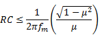
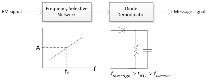
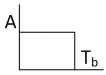
Time constant of Envelope Detector:
If |
|


1. Need for frequency translation
a. To achieve practical lengths of antennas.
b. Reduces the ratio of highest to the lowest frequency band in the signal.
2. Method of frequency translation
a. Multiplication with sinusoidal time signal of higher frequency than the base signal.
3. Recovery of the baseband signal
a. Multiplication with sinusoidal time signal followed by low-pass filtering. [this method is applicable only if the phase of the signal is constant].
4. Multiplier and Mixer
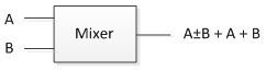
Mixer is about addition
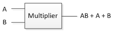
Multiplier is about product
5. Balanced Modulator and Amplitude Modulator.
Amplitude Modulator is a multiplier and is a non-linear device (eg. Class-C amplifiers)
Balanced modulator is a pair of multipliers followed by an adder. Its output is multiplication of input only (none of the input appear individually at the output).
Hilbert Transform(HT)
In the field of signal processing:
1. Hilbert Transform of a signal introduces phase shift of 900 in all the signal components.
2. Hilbert Transform gives analytic representation of a signal
HT
of a signal ![]() is defined as
is defined as
![]()

Instantaneous
frequency ![]()
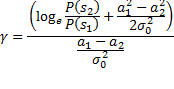
1. Phase Modulated signal
·
![]()
·
Maximum frequency deviation =![]()
It is the positive maximum deviation of the phase of the modulated signal from the phase of the carrier.
·
Modulation index for sinusoidal message signal =![]()
·
Modulation index for non-sinusoidal message signal ![]()
2. Frequency Modulated signal
·
![]()
·
Instantaneous phase is ![]()
·
Instantaneous frequency is ![]()
·
Maximum frequency deviation ![]() when the message
signal is
when the message
signal is ![]()
It is the positive maximum deviation of the frequency of the modulated signal from the frequency of the carrier.
·
Carrier Swing ![]()
It is the maximum deviation of the frequency of the modulated signal from the frequency of the carrier.
·
Modulation index for sinusoidal message signal =![]()
·
Modulation percent ![]()
·
Bandwidth = ![]()
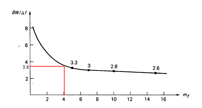
· Bandwidth can also be calculated using Schwartz Curve
·
Modulation index for non-sinusoidal message signal ![]()
· If message signal is sinusoidal then modulated signal can be expressed as
![]() where
where ![]()
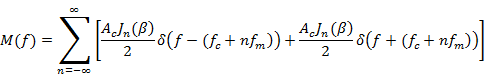
3. Frequency Spectrum of Angle Modulated Signal
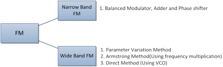
4. Methods of FM Generation
1. Parameter Variation Method
2. Armstrong Method (uses frequency multiplication)
5. Frequency Multiplication and its effect on modulation index and frequency deviation
· n-times frequency multiplication increases the modulation index by n times
· n-times frequency multiplication increases the frequency deviation by n times
|
Parameters |
Phase Modulation
|
Frequency Modulation
|
|
Modulated Signal |
|
|
|
Instantaneous Phase |
|
|
|
Instantaneous Frequency
|
|
|
|
Deviation |
Phase deviation |
Frequency Deviation |
|
Modulation Index |
|
|
|
Bandwidth |
|
|
|
Narrowband |
|
|
|
Parameters |
PM |
FM |
|
Deviation |
Phase
deviation |
Frequency
deviation |
|
Modulation index |
Modulation
index |
Modulation
index |
|
Bandwidth |
Bandwidth |
Bandwidth |
|
Parameters |
PM |
FM |
|
Deviation |
Phase deviation unchanged |
Frequency deviation |
|
Modulation index |
Modulation index unchanged |
Modulation
index |
|
Bandwidth |
Bandwidth unchanged |
Bandwidth unchanged |
Say
modulation index = 4 then from the curve ![]()
|
Criteria |
Type of FM |
Bandwidth |
|
modulation
index |
Wideband FM |
Bandwidth |
|
modulation
index |
Narrowband FM |
Bandwidth |
Narrow band is comparable to Amplitude modulation
If
the modulating signal is not sinusoidal then it falls under the category of
arbitrary modulation of carrier . For such system modulation index is called
Deviation ratio ![]()
![]()
![]() is the bandwidth of
modulating signal.
is the bandwidth of
modulating signal.
Bandwidth
of the modulated signal ![]()
|
SNR- FM |
|
|
|
SNR- PM |
|
|
|
SNR- AM |
|
|
·
![]()
·
![]() if
if ![]()
![]()
·
![]() if
if ![]()

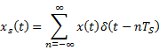
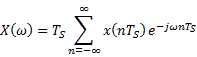
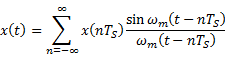
Transmission of bitstreams using M-ary multilevel waveforms


|
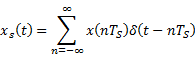
Let us start
with a signal
OR
|
The Fourier
transform of
OR
|
|
Regeneration
of
Thus
|
Substituting
Taking Inverse Fourier transform gives
|

In quantization process actual value of the sampled signal is replaced by a quantized value.

|
Type of Modulation |
Quantization Error (mean squared) |
|
PCM |
|
|
Delta |
|
1.
Let analog signal vary form ![]() to
to ![]()
2.
Divide the signal swing into ![]() intervals (here
intervals (here ![]() )
)
3.
Hence Step size of each interval is ![]()
4. In any interval the value of the signal is approximated to midpoint of that interval.
5.
SNR =![]()
|
If
quantization error |
|
|
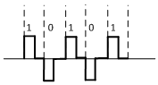
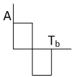
Line Coding |
|
·
If
·
Let us say that a stream of 0's and 1's is spewed into the
channel. If the time period of the pulse used to transmit
So
the channel gets pulse at time
The
receiver also checks for pulses at
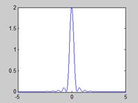
ISI occurs if pulse spread (which they do in physical channel) and at the time of sampling at receiver they give false output as shown in the figure.
If
the pulse shape is perfect sinc with zero crossing at
Rule
of Thumb: A transmission with bit rate
Using
Raised cosine pulse, roll-off
|
|
Unipolar NRZ |
|
|
|
Unipolar ZR |
|
|
|
Bipolar NRZ |
|
|
|
Bipolar ZR |
|
|
|
AMI |
|


![Machine generated alternative text:
ñoño ft
IL] Lii](Communication_Systems_files/image161.png)

Analog
signal with amplitude range ![]() and maximum
frequency
and maximum
frequency ![]() is PCM encoded using
is PCM encoded using
![]() bits per sample.
The signal is sampled at a rate of
bits per sample.
The signal is sampled at a rate of ![]() and a
and a ![]() multilevel signal is
used for transmission.
multilevel signal is
used for transmission.
|
Number of Levels (L) |
|
|
Step Size (S) |
|
|
Average Quantization Noise Power |
|
|
SNR (db) |
|
|
SNR (in terms
of |
|
|
SNR (in terms of system bandwidth) (db) |
|
|
System
bandwidth |
|
|
Nyquist rate
of sampling a PCM Encoded signal |
|
|
Bit rate of PCM Encoded signal |
|
|
Channel Bandwidth |
|

Analog
signal ![]() with bandwidth
with bandwidth ![]() is sampled at
is sampled at ![]() and delta modulated
with step size
and delta modulated
with step size ![]() and a post
construction filter with bandwidth
and a post
construction filter with bandwidth ![]() is used
is used
|
Maximum quantization error |
|
|
Step size to avoid Slope overload |
|
|
SNR (db) with postconstruction filter |
|
|
SNR (db) taking without postconstruction filter |
|
Random Variables are functions that map events (sample points) to real valued numbers.

A
random variable is a ![]() which maps sample
points to a real valued number. Simply put
which maps sample
points to a real valued number. Simply put ![]()
· In the context of random variable sample space is also known as 'domain'.
·
The values taken by ![]() is called the 'range
of
is called the 'range
of ![]() '.
'.

|
To calculate
Probability of a random variable
|
|
|
Properties of |
1.
2.
3.
4.
5.
6.
|
|
Properties of |
1.
2.
3.
|
|
Properties of |
1.
2.
3.
|

|
Conditional Probability |
If |
|
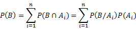
Total Probability : Let there be a
sample space |
|
|
Bayes Theorem
|
|
Let ![]() and
and
![]() represent sent and
receive respectively and it is given
represent sent and
receive respectively and it is given
|
|
Probability
that a |
|
|
Probability that a 0 was received |
|
|
Probability
that a |
|
|
Probability
that a |
|
|
|
|
|
|
|
|
|
|
|
|

|
Calculate |
Solution |
|
P( |
|
|
|
|
|
|
|
|
|
|
|
|
|
|
|
|
|
|
|
|
|
|
|
Probability of
error |
|
|
Probability
of zero error
|
|
|
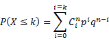
Binomial Distribution
Discrete RV function |
|
If
|
|
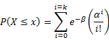
Poisson
Distribution
Discrete RV function
|
|
|
|
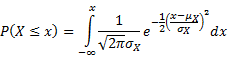
Normal Distribution
Continuous RV function
|
|
|
|
Exponential Distribution
Continuous RV function |
|
|

|
Property |
Using probability Mass Function |
Using probability density function |
|
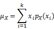
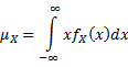
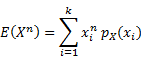
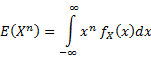
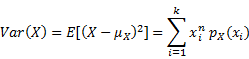
Mean |
|
|
|
n-Moment |
|
|
|
Variance |
|
|
|
Correlation |
|
|
|
Covariance |
|
|
If ![]() then
then ![]() ,
, ![]() and
and ![]() are said to be
uncorrelated.
are said to be
uncorrelated.
If ![]() then
then ![]() and
and ![]() are
independent.
are
independent.
If ![]() and
and ![]() are
independent then
are
independent then ![]() but the converse is
not necessarily true.
but the converse is
not necessarily true.
If ![]() and
and ![]() are
independent then
are
independent then ![]()
Moment
Generating function : ![]() . The
. The ![]() moment is define as
moment is define as
![]()
![]()
![]()

|
Probability of Error |
1.
2.
|
|
|
The detector outputs The detector outputs
Since |
|
What is the probability that |
|
|
What is the probability that |
|
|
What is the probability of bit error |
|
|
Evaluation of threshold value
|
|

|
|
1.
2.
3.
4. All sample functions is called an ensemble
The values that a random process can take is called state-space. It could be discrete-state or continuous-state.
The time line of a random process is called index set. It could be discrete-parameter or continuous parameter corresponding to discrete or continuous time respectively.
|
|
Density
function of Random process : The |
|
|
Ensemble
Average (mean) of |
|
|
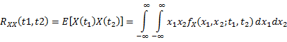
Autocorrelation
|
|
|
Covariance |
|
|
Strict Sense
Stationary |
A
random process
|
|
Wide Sense
Stationary |
A
random process
1.
2.
|
|
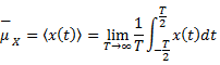
Time-average
mean |
|
|
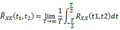
Time-average
Autocorrelation |
|
|
Ergodic Random Process |
A random process is called ergodic if ensemble average equals time-average |

|
Autocorrelation |
Cross-correlation |
Auto-covariance |
Cross-covariance |
|
1. 2. 3. 4.
|
1. If 2.
|
1.
|
1. |
Passing a random process through an LTI system

|
Properties of Autocorrelation Function |
Properties of Power Spectral Density (watts/Hz) |
|
1.
2.
3.
4.
|
1.
2.
3.
4.
|
|
Valid Autocorrelation Function |
Invalid Autocorrelation Function |
||||||
|
|
||||||
|
Valid Power Spectral Density
|
Invalid Power Spectral Density
|


![Machine generated alternative text:
2r
x(t)= Acos—t+
congII ‘
Random P%. (U.tnem
DIribuIo.iI
E ¡me Averaging
First Moment Ensemble Averaging First Moment
Zlt
(1) (2ff
IfAcr+.)dt_0] — Acos%_t+Ø)dO
n
jo ___________________________
o o
Time Averaging
Second Moment Ensemble Averaging Second Moment
r
1) 2n AZ
T f p(,)xz()_f (2 Azcos0( r4)d_ 2
IfA2co52(Ttø)d
lo](Communication_Systems_files/image383.png)
|
|
||||||||||||
|
|
|
|||||||||||
|
|
|
|||||||||||
|
|


|
Modulation System |
General Arrangement of Receiver System |
|
Base band System |
|
|
Amplitude Modulated System |
|
|
Angle Modulated System |
|


|
Noise in Baseband Communication System
1. Receiver is
an Ideal Low-pass filter with bandwidth 2. Message signal
3. For sake of
simplicity substitute
|
Synchronous Detection
|
|
|
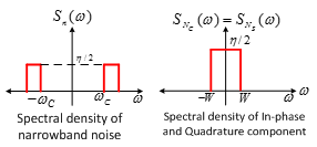
Noise in Amplitude Modulated DSB System
1. Receiver is a
combination of Ideal Band-pass filter with bandwidth 2. Message signal
3. For sake of
simplicity substitute
Bandpass filter is also known as predetection filter.
|
Synchronous Detection
|
|
|
Noise in Amplitude Modulated SSB System
1. Receiver is a
combination of Ideal Band-pass filter , demodulator
and an Ideal Low-pass filter with bandwidth 2. Message signal
3. For sake of
simplicity substitute
|
Synchronous Detection
|
|
|
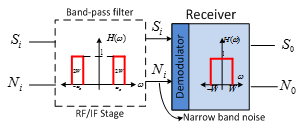
Noise in Normal Amplitude Modulated System |
Synchronous Detection
Envelope Detection
|
The phenomenon
where degrades very rapidly using envelope detection is called threshold effect.
For sinusoidal
signal and 100% modulation
|
|
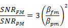
SNR in PM |
|
|
|
SNR in PM |
|
|


Assuming
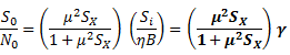
that ![]() is a random process
message signal with average power
is a random process
message signal with average power ![]() . The SNR of some of
the common modulation schemes
. The SNR of some of
the common modulation schemes
|
Normal AM Signal with message bandwidth |
|
After synchronous demodulation
|
|
DSB AM Signal with message bandwidth |
|
After Synchronous demodulation
|
|
SSB(Lower Side
band) AM Signal with message bandwidth
OR
SSB(Upper Side
band) AM Signal with message bandwidth |
OR
|
After Synchronous demodulation
|
|
PM Signal |
|
|
|
FM Signal |
|
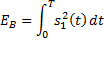
* The complicated expression for |
|
The
transfer function of a matched filter
|
|
|
A matched filter produces maximum SNR at the output for a given signal at its input |
|

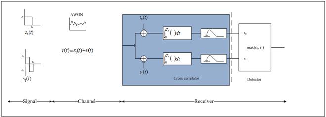
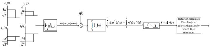
· Lets see what happens step by step:
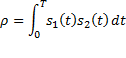
a. si(t) is transmitted [ it could be s0(t) or s1(t)].
b. si(t) enters the channel and get corrupted by noise. The source of noise could be anything. Mathematically this noise is modeled as thermal noise. All that we know about this noise is its power-spectral density. Let say the corrupted signal is r(t).
c. r(t) hits the correlator.
d. Correlator integrates and its output is sampled at Tb.
Case1: s0(t) is transmitted
· r(t) is a random process because n(t) is a Gaussian random process.
· r(t) after passing through correlator and sampler gives a random variable.
· r0 is a random variable and r1 is also a random variable.
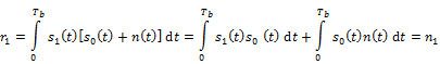
mean(![]()
![]()
This is the point
where things get a little complicated. I cannot express ![]()
![]() like this [
like this [![]() So what I am looking at is
So what I am looking at is ![]() .
.
Autocorrelation is defined just for this kind of expression.
![]()
Finally ![]()
·
Mean
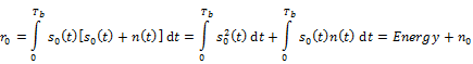
(r0)=Energy of s0(t) ;Var(r0)=![]() Energy of s0(t)
Energy of s0(t)
·
Mean
(r1)=0 ;Var(r1)=![]() Energy of s1(t)
Energy of s1(t)
·
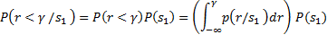
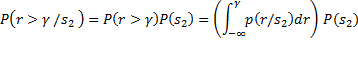
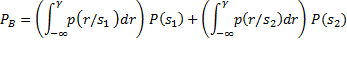
Probability
density of r0 when s0(t) is transmitted is ![]()
·
Probability
density of r1 when s0(t) is transmitted is ![]()
·
Calculation
of probability of error: If ![]() is transmitted and the output of the
detector is
is transmitted and the output of the
detector is ![]() then an error has occurred. Detector
would make this mistake only when the value of
then an error has occurred. Detector
would make this mistake only when the value of ![]() is greater than [
is greater than [![]() +
+![]() which implies that
which implies that ![]()
·
![]()
·
![]() is again a random variable. Now we have
to come up with ways to finds its probability density in order to evaluate
is again a random variable. Now we have
to come up with ways to finds its probability density in order to evaluate ![]()
·
Mean![]() =mean(
=mean(![]() )-mean(
)-mean(![]() )=0
)=0
·
![]()
![]()
(Since both the signals here have equal energy)
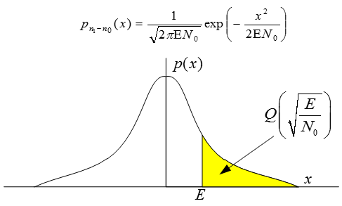
· 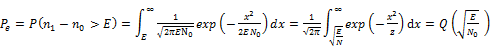
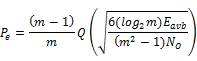
Greater the magnitude of the argument of error function Q the smaller its value. So by increasing the energy of the signal probability of error could be reduced.
Case2: s1(t) is transmitted
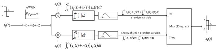
· Probability density
of r0 when s0(t) is transmitted is ![]()
· Probability density
of r1 when s0(t) is transmitted is ![]()
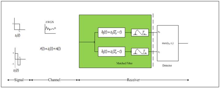
· Base-band signal transmission receiver containing matched-filter.
Case1: s0(t) is transmitted
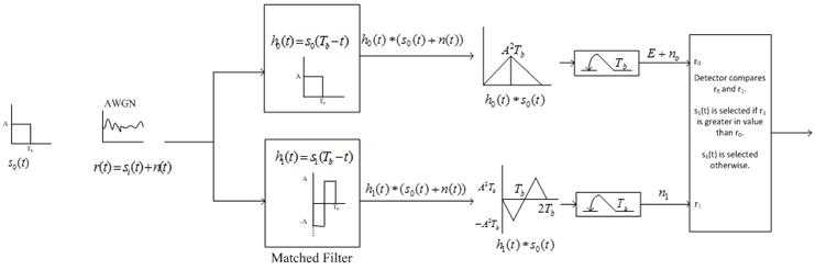
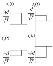
· 4-amplitude signal
|
Signal |
|
Waveforms |
Probability of error in terms of Error function Q |
Signal Energy per bit |
|
|
Binary Orthogonal |
|
|
|
|
No of correlators in the receiver =2 |
|
Binary Antipodal |
|
or
|
3db better than orthogonal signal for the same signal energy |
|
No of correlators in the receiver =1 |
|
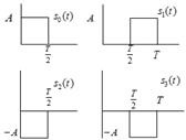
4-amplitude signals (one-dimensional signals) |
g(t) is unit energy pulse
|
|
|
Each symbol has different engery.
Average
symbol energy
Average
bit energy |
No of correlators in the receiver =1 |
|
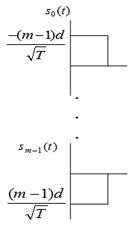
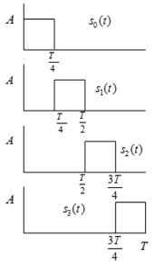
m-amplitude signals (one-dimensional signals) |
g(t) is unit energy pulse
|
|
|
Each symbol has different engery.
Average
symbol energy
Average
bit energy |
No of correlators in the receiver = 1 |
|
Orthogonal Multi-dimensional signal |
|
|
|
No of correlators in the receiver = m |
|
|
Biorthogonal |
No of signals= m
|
|
|
No of
correlators in the receiver |


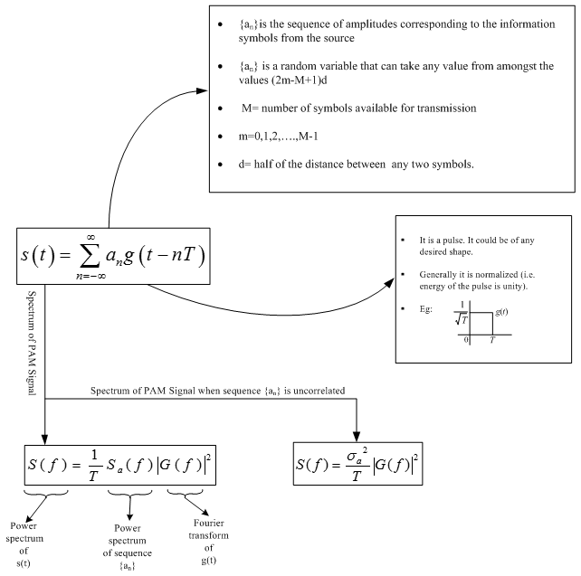
· Expression for a PAM signal s(t) with symbol interval T
·
The
point to understand here is that ![]() is a random variable and
is a random variable and ![]() is a sample function of a random
process S(t). To determine the spectral characteristics of random process we must
evaluate its power spectrum and here autocorrelation comes into the picture.
is a sample function of a random
process S(t). To determine the spectral characteristics of random process we must
evaluate its power spectrum and here autocorrelation comes into the picture.
|
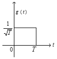
Symbol source |
Transmitter Pulse
|
Spectrum of symbol source |
Fourier Transform of Transmitter pulse |
Spectrum
|
Plot of spectrum |
|
|
|
|
|
|
|
|
|
|
|
|
|
T=1
|
|
|
|
|
|
|
T=1
|
Frequency
response of some communication channels like telephone channels and some radio
channels can be modeled as ![]()
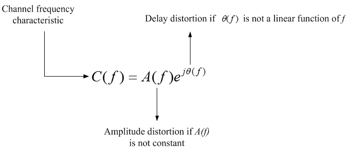
·
Group delay is defined as ![]()
· Group delay is also known as envelope delay.
· Group delay not constant means delay distortion.
· Delay distortion causes intersymbol interference(ISI).
· Use of equalizers or filters reduce ISI.
Some channels like shortwave propagation through ionosphere, mobile cellular radio and tropospheric scatter are modeled using scattering function.