Contents
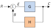
Canonical Form of Feedback Network
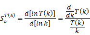
Sensitivity of some simple transfer functions
Steady State Error and coefficients
|
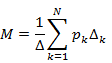
Mason's Gain Formula |
|
combination of 2 non-touching loops)
combination of 3 non-touching loops)
combination of 4 non-touching loops) …..
the
combination of 2 non-touching loops not touching the forward path)
combination of 3 non-touching loops not touching the forward path) …..
|
|
|
|
||||||||||||||||||
|
|
|
|
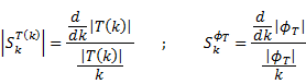
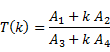
Sensitivity
of a system with transfer function |
|
|
|
|
|
Sensitivity w.r.t to magnitude and phase |
|
|
Sensitivity overall |
|
|
|
|
|
|
|
|
Unity feedback System: Here closed loop transfer function can be expressed as a function of open loop transfer function.
Sensitivity of
|
This shows that a closed system is stable =1, even as open loop gain is infinity. |

|
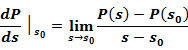
Steady State
Error |
|
This is direct application of final value theorem.
|
|
Position Error Coefficient |
|
|
|
Velocity Error Coefficient |
|
|
|
Acceleration Error Coefficient |
|
|
The type of open loop transfer function is important in determining error due to various signals
|
Type |
0 |
1 |
2 |
3 |
4 |
|
Unit Step |
|
|
|
|
|
|
Ramp |
|
|
|
|
|
|
Parabolic |
|
|
|
|
|
|
Type |
0 |
1 |
2 |
3 |
4 |
|
Unit Step |
|
|
|
|
|
|
Ramp |
|
|
|
|
|
|
Parabolic |
|
|
|
|
|
|
Gain Margin : Reciprocal of gain at phase crossover frequency.
Phase
crossover frequency is the frequency at which phase is |
|
|
Phase Margin : Amount of phase that can be added at gain crossover frequency.
Grain crossover frequency is the frequency at which gain is unity |
Phase Margin =
|
|
Resonant Peak : It is the maximum value of the magnitude of the closed-loop transfer function. |
|
|
Resonant Frequency : It is the frequency at which resonant peak occurs. |
|
|
Cut-off rate : It is the frequency rate at which magnitude ratio changes after cut-off frequency |
|
|
Bandwidth : |
|
|
Delay time : Speed of response |
|
1. NP Gives measure of stability of closed loop systems from open-loop transfer function.
2. NP is an extension of Polar plot.
3. Nyquist Plot is the mapping of Nyquist Path into ![]() function plane.
function plane.

1.
In control system
analysis Nyquist Plot is drawn is for the function ![]()
2. ![]() is the denominator of the closed loop transfer function(CLTF) of
a system.
is the denominator of the closed loop transfer function(CLTF) of
a system.
3. The roots(or zeros) of ![]() determines the stability of CLTF.
determines the stability of CLTF.
4. For stability of CLTF, the roots of ![]() must not lie in the right half s plane.
must not lie in the right half s plane.
If P is the number of poles
of GH(s) inside the Nyquist Path and N is the number of encirclement of ![]() point
by the Nyquist Plot then the CLTF is stable if
point
by the Nyquist Plot then the CLTF is stable if ![]() is
zero where
is
zero where ![]() is
the number of zeros of
is
the number of zeros of ![]() that lie inside the Nyquist Path.
that lie inside the Nyquist Path.
|
Mapping of |
|
|
Plotting of |
|
|
Analyticity of
|
If
For e.g. |
![Machine generated alternative text:
ja, Im[P(s)]
Mapping
ð
¡L Ps1)
0• 4 Re[P(s)]
s-plane P(s)-plane
s=cY+jú) P(s) =Re[P(s)]±jlm[P(s)]](Control%20Systems_files/image073.png)
![Machine generated alternative text:
1m [P(s)]
ja)
- -
-
C 4 ( Re[P(s)J
j3
54](Control%20Systems_files/image075.png)
|
If
the angle between the curves
|
|

|
|
|
![Machine generated alternative text:
co=O
(û = — X’
(û -Plane P(ja,)—Plane
Re[P(fto)]
w = X
Irn[P(jw)]](Control%20Systems_files/image089.jpg)
|
·
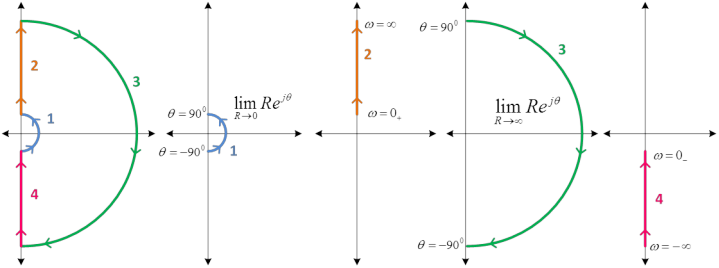
A Nyquist path
encloses the entire right half of the s-plane. If any pole(s) or zero(s) lie
on the
·
Path components 2, 3
and 4 are common to any Nyquist Path but the number of appearances of path
component 1 depends on the number of poles or zeros on the ·
Nyquist Path is
mapped into
|
|
|
|
|
Nyquist Path |
|
Here Nyquist path is the entire RHS s-plane. A pole lies in the LHS s-plane.
This pole doesn't lie inside Nyquist Path.
|
|
|
Here
Nyquist path is the entire RHS s-plane with detours around the poles on
A pole and a zero lies in the RHS s-plane.
|
|


|
|
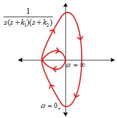
Nyquist Plot |
|
Nyquist Plot |
|
|
|
|
|
|
|
|
|
|
|
|
|
Lead Network |
|
|
|
|
Lag Network |
|