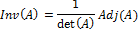
Methods of finding Inverse of a matrix:
Methods to find the rank of a matrix
Procedure to find the Normal form of a matrix
Derivative of Implicit Function
Euler's Theorem (Homogenous functions)
Differentiate using Leibnitz's Rule
Common Trigonometric Functions
ORDINARY DIFFERENTIAL EQUATIONS
Understanding Linearity of ODE
Non Exact Differential Equation
Linear / Non-Linear First Order DE
Linear Second/Higher Order DE (LODE)
Non Homogenous LHODE (VC) reducible to LHODE (CC)
Theorem of Total Probability (Rule of Elimination)
Roots of Non-linear (Transcendental) Equations
Methods of solving non-linear equations / Finding roots of non-linear equations
Newton's Interpolation Formula
Newton's Divided Difference Formula
Lagranges Interpolation Formula
Numerical Solutions of First Order ODE
Milne's Predictor Corrector method
Piccard's Successive Approximation
Adam-Bashforth-Moulton's Method (ABM)
Some common curves in parametric form
Line Integral of normal functions
Surface Integral of vector functions/fields
Surface Integral of normal functions
Surface Integral of normal functions (SURFACE PARAMETERIZED)
Direct Evaluation of Surface Integrals
Evaluation of Surface Integrals
How use solution directly in some expression
1)
If A is a ![]() matrix then the reduced row-echelon form of
the matrix will either contain at least one row of all zeroes or it will be
matrix then the reduced row-echelon form of
the matrix will either contain at least one row of all zeroes or it will be ![]() the
the ![]() identity matrix.
identity matrix.
2)
If A and B are both ![]() matrices then we say that A = B provided
corresponding entries from each matrix are equal. In other words, A = B
provided
matrices then we say that A = B provided
corresponding entries from each matrix are equal. In other words, A = B
provided ![]() for all i and j.
for all i and j.
Matrices of different sizes cannot be compared.
3) If ![]() and B are both
and B are both ![]() matrices then
matrices then ![]() is a new
is a new ![]() matrix that is found
by adding/subtracting corresponding entries from each matrix.
matrix that is found
by adding/subtracting corresponding entries from each matrix.
![]()
Matrices of different sizes cannot be added or subtracted
4)
If A is any matrix and
c is any number then the product (or scalar multiple) ![]() , is a new matrix of the same size as A
and it’s entries are found by multiplying the original entries of A by c.
, is a new matrix of the same size as A
and it’s entries are found by multiplying the original entries of A by c.
In other
words ![]() for all i and j.
for all i and j.
5) Assuming that A and B are appropriately sized so that AB is defined then,
1. The ![]() row of AB is given by the matrix product:
[
row of AB is given by the matrix product:
[![]() row of A]B
row of A]B
2. The ![]() column of AB is given by the matrix
product: A[
column of AB is given by the matrix
product: A[![]() column of B]
column of B]
6)
If A is a ![]() matrix then the transpose of A, denoted
by
matrix then the transpose of A, denoted
by ![]() is an
is an ![]() matrix that is obtained by interchanging
the rows and columns of A.
matrix that is obtained by interchanging
the rows and columns of A.
7)
If A is a square
matrix of size ![]() then the trace of A, denoted by
then the trace of A, denoted by ![]() , is the sum of the entries on main
diagonal.
, is the sum of the entries on main
diagonal.
![]()
If A is not square then trace is not defined.
8) ![]() does not always imply
does not always imply
![]() or
or ![]()
![]() with
with ![]() and
and ![]() unlike real number
properties.
unlike real number
properties.
Real number properties may OR may-not apply to matrices.
9)
If
![]() is a
is a ![]() square matrix then
square matrix then
![]()
![]()
![]()
![]() ;
; ![]() ;
; ![]()
10) If A and B are matrices whose sizes are such that given operations are defined and c is a scalar then
![]() ;
; ![]()
![]() ;
; ![]()
11) If A is a square matrix and we can find another matrix of the same size, say B, such that
![]()
Then we call ![]() invertible and we say that B is
an inverse of the matrix A.
invertible and we say that B is
an inverse of the matrix A.
a.
If
we can’t find such a matrix ![]() we call
we call ![]() singular
matrix.
singular
matrix.
b. Inverse of a matrix is unique.
c.
![]()
![]()
d.
![]()
e.
![]()
12) A square matrix is called an elementary matrix if it can be obtained by applying a single elementary row operation to the identity matrix of the same size.
E.g. ![]()
13)
Suppose
A is a ![]() matrix and by performing one row
operation R ( ) it becomes another matrix say B. Now if same row operation R(
) is performed on an identity matrix
matrix and by performing one row
operation R ( ) it becomes another matrix say B. Now if same row operation R(
) is performed on an identity matrix ![]() and it becomes matrix say E ,
then E is called the elementary matrix corresponding to the row operation R( )
and multiplying E and A would give B.
and it becomes matrix say E ,
then E is called the elementary matrix corresponding to the row operation R( )
and multiplying E and A would give B.
14) Suppose ![]() is the elementary matrix associated with
a particular row operation and
is the elementary matrix associated with
a particular row operation and ![]() is the elementary matrix associated with
the inverse operation. Then E is invertible i.e.
is the elementary matrix associated with
the inverse operation. Then E is invertible i.e. ![]()
Suppose that we’ve got two matrices of the same size A and B. If we can reach B by applying a finite number of row operations to A then we call the two matrices row equivalent.
Note that this will also mean that we can reach A from B by applying the inverse operations in the reverse order
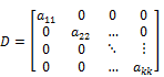
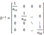
If any diagonal element is zero then the matrix is singular
Upper-Traingular
Matrix= 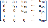
Lower-Traingular
Matrix = 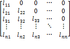
Matrix ![]() is orthogonal if
is orthogonal if ![]()
Matrix ![]() is orthogonal if
is orthogonal if ![]()
Matrices ![]() and
and ![]() are orthogonal if
are orthogonal if ![]()
Matrix ![]() is said to be similar to matrix
is said to be similar to matrix ![]() if
if ![]() can be expressed as
can be expressed as
![]()
where ![]() is some non-singular matrix
is some non-singular matrix
Matrix ![]() is unitary if
is unitary if ![]()
![]() is the complex conjugate of
is the complex conjugate of ![]()
A Hermitian matrix
(also called self-adjoint matrix) is a square matrix with complex entries which
is equal to its own conjugate transpose - i.e. the element in the ![]() row and
row and ![]() column is equal to
the complex conjugate of the element in the
column is equal to
the complex conjugate of the element in the ![]() row and
row and ![]() column, for all
column, for all ![]() and
and ![]()
·
![]()
·
Example:
![]()
· Entries on main diagonal are always real
· A symmetric matrix with all real entries is Hermitian
A Hermitian matrix
with complex entries which is equal to negative of its own conjugate transpose
- i.e the element in the ![]() row and
row and ![]() column is equal to
the negative of complex conjugate of the element in the
column is equal to
the negative of complex conjugate of the element in the ![]() row and
row and ![]() column, for all
column, for all ![]() and
and ![]()
·
![]()
·
E.g.:-
![]()
· Entries on main diagonal are always purely imaginary
·
If
![]() is skew-Hermitian
then
is skew-Hermitian
then ![]() raised to odd power
is skew-Hermitian
raised to odd power
is skew-Hermitian
·
If
![]() is skew-Hermitian
then
is skew-Hermitian
then ![]() raised to even power
is skew-Hermitian
raised to even power
is skew-Hermitian
|
Symmetric |
|
|
|
Skew-Symmetric |
|
|
|
Hermitian |
|
|
|
Skew-Hermitian |
|
|
|
Conjugate-Symmetric |
|
|
|
Conjugate-Anti-Symmetric |
|
Same as Skew-Hermitian |
A matrix ![]() is idempotent if
is idempotent if ![]()
· An idempotent matrix is diagonalizable
· Eigen values are 0 or 1
· Rank of an idempotent matrix = sum of its diagonal elements
A matrix ![]() is Involutory matrix
if
is Involutory matrix
if ![]()
·
If
![]() is involutory then
is involutory then ![]()
·
A
![]() Matrix of the form
Matrix of the form ![]() is always
involutory.
is always
involutory.
A matrix that has exactly one entry of 1 in each row and column and zero elsewhere is called a permutation matrix.
· It is a representation of permutation of numbers
·
Example:-
 is permutation
matrix of the permutation (1,3,2,4)
is permutation
matrix of the permutation (1,3,2,4)
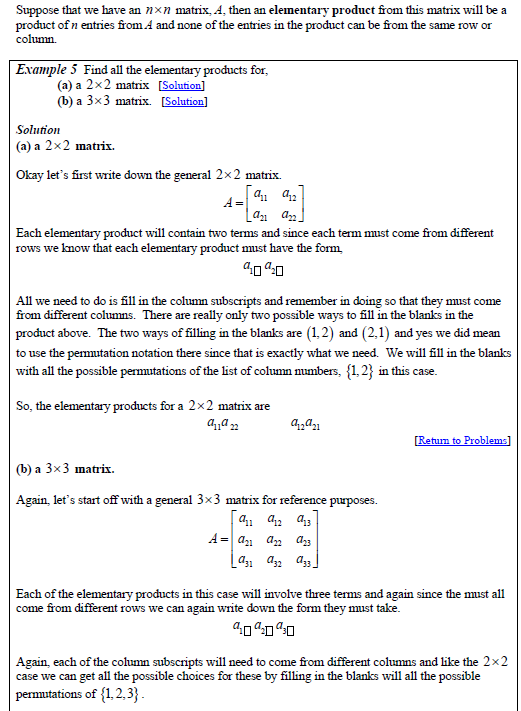
Determinant functions: The determinant function is a function that will associate a real number with a square matrix.
Permutation of integers: An arrangement of integers without repetition and omission.
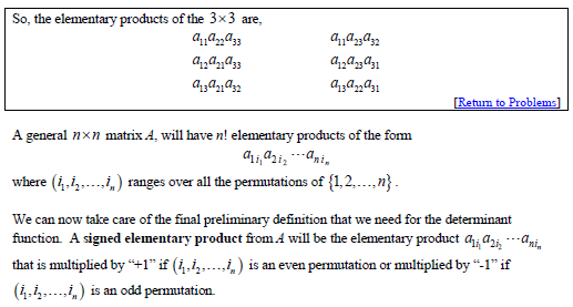
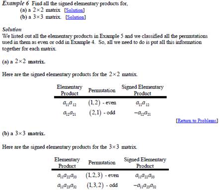
Theorem 1: If
A is square matrix then the determinant function is denoted by ‘det’ and ![]() is defined to be the sum of all the signed elementary products of A.
is defined to be the sum of all the signed elementary products of A.
1.
![]()
2.
![]() {it may be equal
in some cases but not so in general}
{it may be equal
in some cases but not so in general}
3.
![]()
4.
![]()
5.
![]()
6.
![]() …
…![]() if A is a triangular
matrix
if A is a triangular
matrix
7.
If
![]() is the matrix that
results from multiplying a row or column of
is the matrix that
results from multiplying a row or column of ![]() by a scalar c, then
by a scalar c, then ![]()
If ![]() is the matrix that results from
interchanging two rows or two columns of
is the matrix that results from
interchanging two rows or two columns of ![]() then
then ![]()
If ![]() is the matrix that results from adding a
multiple of one row of
is the matrix that results from adding a
multiple of one row of ![]() onto another row of
onto another row of ![]() or adding a multiple of one column of A
onto another column of
or adding a multiple of one column of A
onto another column of ![]() then
then ![]()
|
|
|
|
|
2) Using Cofactor. |
|
|
Rank is the highest order of a non-zero minor of the matrix.
Method-1
· Apply elementary row transformation.
· No of non-zero rows = rank of the matrix.
Method-2
· Find all the minors of the matrix.
· Find the order of non-zero minors.
· The highest order is the rank.
Method-3
·
From
the norm of the matrix ![]()
· Rank = r
· ![]()
· ![]()
· ![]()
· ![]()
· ![]()
[![]() is conjugate
transpose of
is conjugate
transpose of ![]() , conjugate transpose
is the adjoint of any matrix]
, conjugate transpose
is the adjoint of any matrix]
Matrix ![]() is said to be
diagonalizable if there exist a non-singular matrix
is said to be
diagonalizable if there exist a non-singular matrix ![]() such that
such that
![]()
Diagonalization of ![]() is possible if and
only if the Eigen vectors of
is possible if and
only if the Eigen vectors of ![]() are linearly
independent.
are linearly
independent.
Some application of Diagonalization:
1.
Evaluation
of powers of ![]() :
: ![]()
2.
Evaluation
of function ![]() over
over ![]() : If
: If ![]() then
then ![]()
3. Not all matrices are diagonalizable but real symmetric matrix (RSM) are always diagonalizable.
4. Eigen vectors of RSM are always distinct
A matrix is symmetric if ![]() . For example A=
. For example A= 
Skew -Symmetric: ![]() . For example B=
. For example B=
The diagonal elements of a skew symmetric is always zero
Eigenvalues of a real skew symmetric matrix is either zero or purely imaginary
The normal form of a
matrix ![]() is
is ![]() where
where ![]() the rank of the
matrix
the rank of the
matrix ![]()
|
Step 1 : |
|
|
|
Step 2 : |
|
Apply ERT on |
|
Step 3 |
|
Apply ERT on |
|
Step 4 |
|
This form is |
So given a matrix ![]() of rank
of rank ![]() two other non
singular matrices
two other non
singular matrices ![]() and
and ![]() can be found such
that
can be found such
that
![]()
![]()
![]() = square matrix (
= square matrix (![]()
![]() =Eigen vector
=Eigen vector
![]() = Eigen value (scalar)
= Eigen value (scalar)
· Eigenvalues and eigenvectors will always occur in pairs.
·
![]()
·
The
set of all solutions to ![]() is called the
eigenspace of
is called the
eigenspace of ![]() corresponding to λ.
corresponding to λ.
·
Suppose
that λ is an eigenvalue of the matrix A with corresponding
Eigenvector![]() .
.
Then if k is
a positive integer ![]() is an eigenvalue of the matrix
is an eigenvalue of the matrix ![]() with corresponding Eigenvector
with corresponding Eigenvector![]() .
.
·
![]()
·
![]() =
=![]()
·
If
![]() are eigenvectors of
are eigenvectors of ![]() corresponding to the
k distinct eigenvalues
corresponding to the
k distinct eigenvalues![]() then they form a
linearly independent set of vectors.
then they form a
linearly independent set of vectors.
Suppose that ![]() is a square matrix and if there exists an
invertible
is a square matrix and if there exists an
invertible
matrix![]() (of the same size as
(of the same size as ![]() ) such that
) such that ![]() is a diagonal matrix then we call
is a diagonal matrix then we call ![]()
diagonalizable and that P diagonalizes A .(Columns of P are the eigen-vectors of A).
THEOREM 1:
Suppose that A is an n× n non-singular matrix, then the following are equivalent.
(a) A is diagonalizable.
(b) A has n linearly independent Eigen-vectors, which forms the column of the matrix that diagonalizes A.
THEOREM 2:
Suppose that A is an ![]() matrix and that A has n distinct
eigenvalues, then A is diagonalizable.
matrix and that A has n distinct
eigenvalues, then A is diagonalizable.
![]() are the Eigen values
of a square matrix
are the Eigen values
of a square matrix ![]()
|
|
|
Same as that of |
|
|
|
|
|
|
|
|
|
|
|
|
|
|
|
|
· Only Eigen vectors of distinct Eigen values are linearly independent.
· For Diagonalization of a matrix its Eigen vectors should be linearly independent.
Every square matrix ![]() satisfies its
characteristic equation.
satisfies its
characteristic equation.
· It is used in calculating the power of matrices (in place of direct matrix multiplication)
![]()
![]()
![]()
The above system of
equation is ![]()
If B=0 system is Homogenous.
If ![]() system in
Non-Homogenous.
system in
Non-Homogenous.
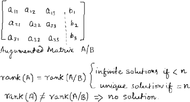
1. Cramer's Method
2. Augmented Matrix Method
3. LU-Decomposition Method
|
Limit |
A function 1. |
|
|
Continuity |
A function 1. 2. |
|
|
Differentiability |
A function
1. 2. Limit
|
|
|
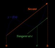
Rolle's Theorem |
If 1. 2. 3. Then there exist a |
|
|
Mean Value Theorem |
If 1. 2.
Then there exist a
|
|
|
Trigonometric |
|
||||||||||||||||||
|
Exponential |
|
||||||||||||||||||
|
Logarithmic |
|
||||||||||||||||||
|
Differentiation |
|
||||||||||||||||||
|
Series |
|
||||||||||||||||||
|
LHospital's Rule
|
|


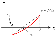
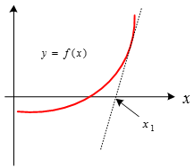
If ![]() is continuous and
derivable in
is continuous and
derivable in ![]() and
and ![]() then there exist at
least one
then there exist at
least one ![]() such that
such that ![]()

If ![]() is a function such
that
is a function such
that ![]() is continuous in the
interval
is continuous in the
interval ![]() and
and ![]() exist in the
interval
exist in the
interval ![]() then Taylor's
theorem says that there exist a number
then Taylor's
theorem says that there exist a number ![]() in the interval
in the interval ![]() and a positive
integer
and a positive
integer ![]() such that
such that
|
|
|
|
|
Cauchy Series |
|
|
|
Lagranges Series |
|
|
|
Maclaurin's Series |
|
|
Convenient form of Taylor's Theorem
![]()
![]()
Taylor Series
expansion of ![]() about the point
about the point ![]() (or in powers of (
(or in powers of (![]() )
)
![]()
|
Total Derivative |
|
|
|
Total Derivative |
|
|
|
First order Derivative of an implicit function
|
|
|
|
Second order partial derivative
of an implicit function |
|
|

|
Homogenous Function |
If homogenous function
|
|
|
Euler's Theorem for Homogenous
function of degree |
|
|
![]() and
and ![]() are two functions of
are two functions of ![]() and
and ![]() . If there is another function such that
. If there is another function such that ![]() then
then ![]() and
and ![]() are said to be functionally dependent.
are said to be functionally dependent.
Test for Functional Dependence
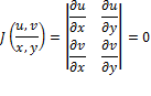
If z=![]() is a function of
is a function of ![]() and
and ![]() then
then ![]()
Using the definition of total derivative
![]()
![]()
Leibnitz's Rule : It
is a rule that gives ![]() order derivative of
product of two functions.
order derivative of
product of two functions.
![]()
|
From Integral Calculus |
|
|
General Leibnitz Rule |
|
|
Leibnitz Rule |
|
|
|
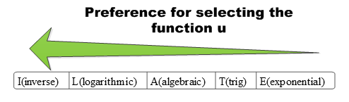
While choosing |
|
|
|
|
|
|
|
|
|
|
|
|
|
|
|
|
|
|
|
|
|
|
|
|
|
|
|
|
|
|
|
|
|
|
|
|
|
|
|
|
|
|
|
|
|
|
|
|
|
|
|
|
|
|
|
|
|
|
|
|
|
|
|
|
|
|
|
|
|
|
|
|
|
|
|
|
|
|
|
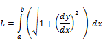
Length |
|
|
|
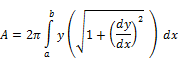
Surface Area of an arc/ curve (obtained by rotating it about x (or y) axis) |
|
|


|
Single Integral |
|
1. It gives the length of the arc 2. It also gives the area between
the arc |
|
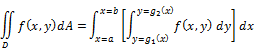
Double Integral |
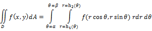
Double Integral (Polar Coordinates)
|
1. It gives the area of the region D.
2. It also gives the volume of the region D |
|
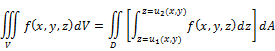
Triple Integral |
|
It gives the volume of the region enclosed by D |
ODE means that there is only one independent variable in the equation
ORDER: order of ODE is the order of the highest derivative appearing in it.
DEGREE: power of the highest order
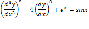
Order = 3
Degree=6
A Differential
Equation where ![]() , the independent
variable and
, the independent
variable and ![]() , the dependent
variable is said to be LINEAR if
, the dependent
variable is said to be LINEAR if
1.
![]() and all its
derivative
and all its
derivative ![]() are of degree one.
are of degree one.
2.
No product term of ![]() and(or) any of its
derivative forms are present.
and(or) any of its
derivative forms are present.
3.
No transcedental functions of ![]() and(or) any of its
derivative are present.
and(or) any of its
derivative are present.
Note: Linearity of a DE depends only on the way the depenedent variable appears in the equation and is independent of the way the independent variable appears in it.
|
Linear ODE |
Non-Linear ODE |
|
|
|
|
|
|
|
|
|
|
Type |
Functional Form |
Examples |
|
Variable Separable Type I |
|
1. 2. 3. 4.
|
|
Variable Separable Type II (requires substitution |
1. Substitute 2. Solve the equations on the lines of Variable Separable Type I
|
1. 2. 3. 4. |
|
Variable Separable Type III (Homogenous ODE reducible to
Variable Separable Type I |
1. 2. Substitute 3. Solve the equations on the
lines of Variable Separable Type I
Note:
|
1. 2. 3. 4.
|
|
Variable Separable Type IV (Non-homogenous ODE reducible to homogenous type reducible to Variable Separable Type I/II) |
1.
2. else
3. Solve
4.
5. Substitute
6. Solve the equations on the
lines of Variable Separable Type I
Note: |
1.
2.
3.
4.
|
|
Exact Differential |
If
|
|
Solution to Exact Differential Equation |
where
or
|
|
Exact DE |
Solution |
|
|
|
|
Steps to Solve Non-Exact Differential Equation
where
|
Step 1: Reduce Non-Exact DE to Exact DE using Integrating Factor (I.F)
Step
2: Solve the Exact DE. Solution is of the form
or
|
|
Type |
Integrating Factor |
|||||||||||||||||||||||||||||||||
|
|
|
|||||||||||||||||||||||||||||||||
|
|
|
|||||||||||||||||||||||||||||||||
|
|
|
|||||||||||||||||||||||||||||||||
|
and
|
|
|||||||||||||||||||||||||||||||||
|
|
|
|||||||||||||||||||||||||||||||||
|
|
where
|
|||||||||||||||||||||||||||||||||
|
Rearranging
|
|
|
A linear first order first degree DE of the form
This DE is known as Leibnitz Linear Equation |
1. Here
2. Also
3. So IF =
4. Solution is
|
||||||
|
A non-linear first order first degree DE of the form
This DE is known as Bernoulli's Equation
|
1. Substitute
2. Equation reduces to Linear PDE
3. Solve using the method described for linear first order DE |
||||||
|
A non-linear first order higher degree DE of the form
|
|
||||||
|
A non-linear first order higher degree DE of the form
This DE is known as Clairaut's Equation |
|
||||||
|
A non-linear first order higher degree DE of the form
This DE is known as Lagrange's Equation
|
|
|
General Linear Higher Order DE |
|
|
Solution of Homogenous LSODE (Constant Coefficients) of the form
or using the notation
|
1. Characteristic Equation is 2. If
|
|
Solution of Homogenous LSODE (Variable Coefficients) of the form
provided the complimentary functions are available
This method is called the method of variation of parameters. |
If the complimentary
solution is
1.
If
2. The particular solution is then given as
3.
|
Note: This method is suitable only for second order DE with variable coefficients. There is no general method for solving higher order DE with variable coefficients.
Solution of Non-Homogenous LSODE (CC) of the form
![]()
![]()
|
1. Characteristic Equation is 2. If
3. Evaluation of Particular
Integral
4. Solution is |
|
Solution of Homogenous LHODE (VC) of the form
or
|
1. Substitute
2. Substitute
where
3. Now the equation is of Homogenous LSODE(CC) form with characteristic
equation of the form
4. Solve the new Homogenous
LHODE(CC) by finding C.F and PI and replace |
|
Solution of Non-Homogenous LHODE (VC) of the form
or
This equation is also known as Cauchy-Euler's Equation |
1. Substitute
2. Substitute
where
3. Now the equation is of Non-Homogenous LSODE(CC) form with
characteristic equation of the form
4. Solve the new Homogenous
LHODE(CC) by finding C.F and PI and replace |
|
Solution of Non-Homogenous LHODE (VC) of the form
or
This equation is also known as Legendre's Equation |
1. Substitute
2. Substitute
where
3. Now the equation is of Non-Homogenous LSODE(CC) form with
characteristic equation of the form
4. Solve the new Homogenous
LHODE(CC) by finding C.F and PI and replace |
There is no general procedure for finding solutions to linear higher order DE with variable coefficients.
|
Some Special Forms |
How to approach for the solution |
|
|
Solve by repeated integration |
|
|
Multiply both sides by
The solution is given by
|
|
Equations not explicitly containing x |
|
|
Equations not explicitly containing y |
|
|
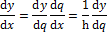
Change of independent variable |
|
|
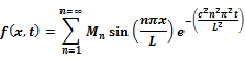
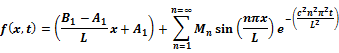
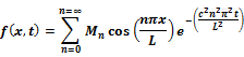
One Dimensional Heat Equation |
Boundary Condition |
Solution |
|
|
Homogenous Boundary Condtion
|
|
|
|
Non-Homogenous Boundary Condtion
|
|
|
|
Homogenous with both ends insulated
|
|


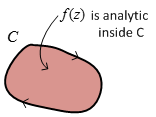
A function ![]() is said to be
analytic at
is said to be
analytic at ![]() if
if ![]() is differentiable at
is differentiable at
![]() and in its
neighbourhood.
and in its
neighbourhood.
![]() is analytic
is analytic ![]()
![]() is differentiable
is differentiable ![]()
![]() is continuous, but
the inverse is not always true.
is continuous, but
the inverse is not always true.
|
Properties of analytic function
|
|
|
If |
|
|
If |
|
|
If |
|
|
Milne's Thompson Method :
If
|
|
|
Cauchy Integral Theorem If
|
|
|
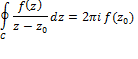
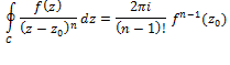
Cauchy Integral Formula If
|
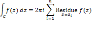
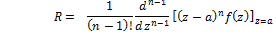
Residue Theorem
If
Residue
|
|
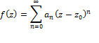
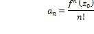
Taylor Series Theorem
If
|
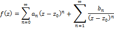
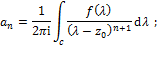
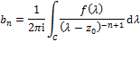
Laurent Series Theorem
If
|


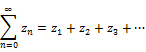
1.
A
sequence of complex numbers is an assignment of a positive integer to a complex
number ![]()
2. A series of complete numbers is the sum of the terms in the sequence. For eg
3.
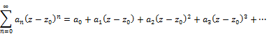
Power
Series: A power series in ![]() is defined as
is defined as
4.
Power
series represent analytic functions. Conversely every analytic function can be
represented as a power series known as the Taylor series. Moreover a function ![]() can be expanded
about a singular point
can be expanded
about a singular point ![]() as a Laurent series
containing both positive and negative integer powers of
as a Laurent series
containing both positive and negative integer powers of ![]()
If an event can be
done in ![]() ways and another
event can be done in
ways and another
event can be done in ![]() ways then both the
events can be done in
ways then both the
events can be done in ![]() ways provided they
cannot be done simultaneously.
ways provided they
cannot be done simultaneously.
If an event can
happen in ![]() ways and another
event can happen in
ways and another
event can happen in ![]() ways then in the
same order they can happen in
ways then in the
same order they can happen in ![]() ways, provided they
do not happen simultaneously.
ways, provided they
do not happen simultaneously.
·
Permutation
of a set of ![]() distinct objects is
an ordered arrangement of these
distinct objects is
an ordered arrangement of these ![]() objects.
objects.
·
Permutation
of a set of ![]() distinct objects
taken
distinct objects
taken ![]() at a time is
at a time is ![]()
·
Permutation
of r objects from a set of n objects with repetition is ![]()
·
Combination
of a set of ![]() distinct objects is
an unordered arrangement of these
distinct objects is
an unordered arrangement of these ![]() objects.
objects.
·
Combination
of a set of ![]() distinct objects
taken
distinct objects
taken ![]() at a time is
at a time is ![]()
·
Combination
of r objects from a set of n objects with repetition is ![]()
·
If
A and B are mutually exclusive then ![]()
·
If
A and B are mutually exclusive then ![]()
·
![]()
·
![]()
·
![]() if A and B are
independent events.
if A and B are
independent events.
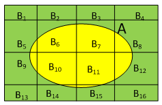
Let ![]() the theorem of total
probability gives
the theorem of total
probability gives
![]()
![]()
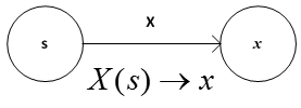
X is a random variable (in fact it is a single valued function) which maps s from the sample space S to a real number x.
·
![]() are different ways
of writing the probability of
are different ways
of writing the probability of ![]()
· f(x) is called the density function.
· ![]()
·
![]()
·
![]()
·
![]()
· F(x) is called the distribution function.
· ![]()
·
Mean
![]()
·
Variance
![]()
·
Variance
![]()
·
![]()
·
Probability
that X will assume a value within k standard deviations of the
mean ![]() is at least
is at least ![]()
·
![]()
·
![]()
· Binomial Distribution
· Mean = np=nq
· Variance = npq
· Hyper-geometric Distribution
·
Mean
= ![]()
· Variance =
· Poisson's Distribution
· ![]()
·
Mean
= ![]()
·
Variance
=![]()
· Normal Distribution
·
![]()
|
Bisection Method |
|
. . .
|
|
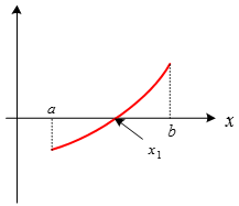
Regula-Falsi
(or Method of chords) |
|
When ├ f(a)>f(b)
|
|
Newton-Raphson Method
(or Method of tangents) |
|
|
A diagonal system is one in which in each equation the coefficient of a different unknown is greater in absolute value than the sum of the absolute values of coefficients of other unknown. For example the system of equations given below is diagonal.
![]()
![]()
![]()
Gauss-Seidel method converges quickly if the system is diagonal.
Steps in Gauss-Seidel method
1. Rewrite the equation as
![]()
![]()
![]()
2. Assume an initial solution (0,0,0)
3.
Evaluate
![]() using
using ![]() Now use the new
Now use the new ![]() and
and ![]() to evaluate
to evaluate ![]() .
.
4.
Now
use ![]() and new
and new ![]() to evaluate
to evaluate ![]()
5. Iterate these steps using new calculated values till desired approximation is reached.
6. If the system is not diagonal, Gauss-Seidel method may or may not converge.
Forward difference is defined as
![]()
·
![]()
·
![]()
|
|
|
|
|
|
|
|
|
|
|
|
|
|
|
|
|
|
|
|
|
|
|
|
|
|
|
|
|
|
|
|
|
|
|
|
|
|
|
|
|
|
|
|
|
|
|
|
|
|
|
|
|
|
|
|
|
|
|
|
|
|
|
|
|
|
|
|
|
|
Backward difference is defined as
![]()
|
|
|
|
|
|
|
|
|
|
|
|
|
|
|
|
|
|
|
|
|
|
|
|
|
|
|
|
|
|
|
|
|
|
|
|
|
|
|
|
|
|
|
|
|
|
|
|
|
|
|
|
|
|
|
|
|
|
|
|
|
|
|
|
|
|
|
|
|
|
|
x |
y |
|
|
|
|
|
|
|
|
|
|
|
|
|
|
|
|
|
|
|
|
|
|
|
|
|
|
|
|
|
|
|
|
|
|
|
|
|
|
|
|
|
|
|
|
|
|
|
|
|
|
|
|
|
|
|
|
|
|
|
|
|
|
|
|
|
|
|
|
|
|
|
|
|
|
|
|
|
|
|
|
|
|
|
|
|
|
|
|
|
|
|
|
|
|
|
|
|
|
|
|
|
|
|
|
|
|
|
|
|
|
|
|
|
|
|
|
|
|
|
|
|
|
|
|
|
|
|
|
|
|
|
|
|
|
|
|
|
|
|
|
|
|
|
|
|
|
|
|
|
|
|
|
|
|
|
|
|
|
|
|
|
|
|
|
|
|
|
|
|
|
|
|
|
|
|
|
|
|
|
|
|
|
|
|
|
|
|
|
|
|
|
|
|
|
|
Divided difference is defined as
![]()
For example
a.
![]()
b.
![]()
·
Divided
difference formula is used for interpolating data sets where the independent
data points are unequally spaced i.e. ![]()
·
But
when the points are equally spaced i.e. ![]() it reduces to
forward/backward difference formula
it reduces to
forward/backward difference formula ![]()
Examples:
1.
![]()
2.
![]()
|
|
|
|
|
|
|
|
|
|
|
|
|
|
|
|
|
|
|
|
|
|
|
|
|
|
|
|
|
|
|
|
|
|
|
|
|
|
|
|
|
|
|
|
|
|
|
|
|
|
|
|
|
|
|
|
|
|
|
|
|
|
|
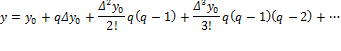
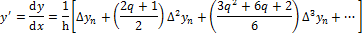
Newtons Forward Interpolation Formula
![]()
|
|
|
|
|
|
|
|
|
|
|
|
|
|
|
|
|
|
|
|
|
|
|
|
|
|
|
|
|
|
|
|
|
|
|
|
|
|
|
|
|
|
|
|
|
|
|
|
|
|
|
|
|
|
|
|
|
|
|
|
|
|
|
|
|
|
|
|
|
|
h= is the uniform distance betwen the data points.
q= a variable introduced to simplify expressions.
![]()
![]()
Newtons Backward Interpolation Formula
![]()
|
|
|
|
|
|
|
|
|
|
|
|
|
|
|
|
|
|
|
|
|
|
|
|
|
|
|
|
|
|
|
|
|
|
|
|
|
|
|
|
|
|
|
|
|
|
|
|
|
|
. . . |
. . . |
|
|
|
|
|
|
|
|
|
|
|
|
|
|
|
|
|
|
h= is the uniform distance betwen the data points.
q= a variable introduced to simplify expressions.
![]()
![]()
Newton's divided difference interpolation formula
![]()
|
|
|
|
|
|
|
|
|
|
|
|
|
|
|
|
|
|
|
|
|
|
|
|
|
|
|
|
|
|
|
|
|
|
|
|
|
|
|
|
|
|
|
|
|
|
|
|
|
|
|
|
|
|
|
|
|
|
|
|
|
|
|
Gaussian Interpolation Formula
|
x |
y |
|
|
|
|
|
|
|
|
|
|
|
|
|
|
|
|
|
|
|
|
|
|
|
|
|
|
|
|
|
|
|
|
|
|
|
|
|
|
|
|
|
|
|
|
|
|
|
|
|
|
|
|
|
|
|
|
|
|
|
|
|
|
|
|
|
|
|
|
|
|
|
|
|
|
|
|
|
|
|
|
|
|
|
|
|
|
|
|
|
|
|
|
|
|
|
|
|
|
|
|
|
|
|
|
|
|
|
|
|
|
|
|
|
|
|
|
|
|
|
|
|
|
|
|
|
|
|
|
|
|
|
|
|
|
|
|
|
|
|
|
|
|
|
|
|
|
|
|
|
|
|
|
|
|
|
|
|
|
|
|
|
|
|
|
|
|
|
|
|
|
|
|
|
|
|
|
|
|
|
|
|
|
|
|
|
|
|
|
|
|
|
|
|
|
|
|
|
|
|
|
|
|
|
|
|
|
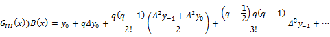
Gaussian Interpolation Formula I
![]()
Gaussian Interpolation Formula II
![]()
Gaussian Interpolation Formula III
![]()
Stirling
Interpolation Formula (Arithmetic mean of ![]() and
and ![]()
![]()
Bessel's
Interpolation Formula (Arithmetic mean of ![]() and
and
|
|
|
|
|
|
|
... |
|
|
|
|
|
|
|
|
... |
|
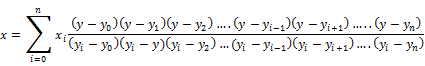
Lagranges interpolation formula is given by
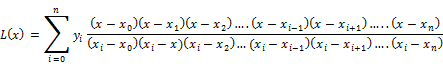
For the given set of data points Lagranges polynomial can be written as
|
|
|
|
|
|
|
|
|
|
![]()
Lagranges inverse interpolation formula is
In spline
interpolation a polynomial called spline S(x) is assigned to each sub interval ![]() and
and ![]()
|
|
|
|
|
... |
|
|
|
|
|
... |
|
Linear Spline |
|
Discontinuous first derivate at the inner knots. |
|
Quadratic Spline |
|
Continuous first derivate at the inner knots.
End points are connected with straight lines. |
|
Cubic Spline |
|
Continuous first and second derivate at the inner knots.
End points are connected with curves |
So a set of n+1 data
points with n sub-intervals would have a different spline polynomial say ![]() for each
sub-interval.
for each
sub-interval.
Differentiating the polynomial ![]() formed using forward interpolation gives
the differentiated polynomial
formed using forward interpolation gives
the differentiated polynomial ![]()
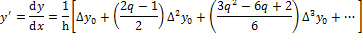
With backward interpolation
The error between interpolated values and actual values is large in case of differentiation than for a polynomial function.
![]()
|
|
|
|
|
... |
|
|
|
|
|
|
... |
|
|
Trapezoidal Rule (n=1) |
|
|
Simpsons |
|
|
Simpson's |
|
|
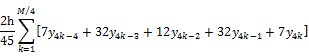
Weddle's Rule (n=6) |
|
|
Boole's Rule |
|
In all the above methods the general rule is to replace the tabulated points with a polynomial function and then carry out its integration. In other words the polynomial is an interpolation function evaluated using Newton's forward (or backward ) interpolation formula. Now if there are large data points then the polynomial becomes oscillatory.
Piecewise interpolation is about finding a separate polynomial for each subinterval rather than for the whole set of data points. These functions are called splines.
1. Taylor's power series method
2. Euler's method
3. Modified Euler's method
4. Runge-Kutta 4th order method
1. Milne's predictor corrector method
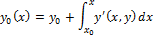
2. Picard's successive approximation method
3. Adam-Bashforth-Moulton method
Taylor series about a point ![]() is given by
is given by

Solve ![]() Given
Given ![]()
Sol : From the given equation we have ![]()
Using Taylor's series about ![]() we have
we have ![]()
Substituting we get the solution ![]()
![]()
· Euler's method does not give us analytical expression of y in terms of x, but it gives the value of y at any point x.
Solve ![]() . Given
. Given ![]() and use step size of
and use step size of
![]() and find
and find ![]()
Sol:
|
|
xi |
|
|
|
|
0 |
0 |
100 |
-1 |
75 |
|
1 |
25 |
75 |
-0.75 |
56.25 |
|
2 |
50 |
56.25 |
-0.5625 |
42.1875 |
|
3 |
75 |
42.18 |
-04218 |
31.63 |
|
4 |
100 |
31.63 |
|
|
![]()
Predictor Formula : ![]()
Corrector Formula : ![]()
Solve ![]() . Given
. Given ![]() , use step size of
, use step size of ![]() Find
Find ![]()
Sol:
|
|
xi |
|
|
|
|
|
|
0 |
0 |
100 |
-1 |
75 |
-0.75 |
78.125 |
|
1 |
25 |
78.125 |
-0.5859 |
58.59 |
-0.5859 |
61.034 |
|
2 |
50 |
61.034 |
-0.6103 |
45.77 |
-0.4577 |
47.68 |
|
3 |
75 |
47.68 |
-0.4768 |
35.76 |
-0.3576 |
37.25 |
|
4 |
100 |
37.25 |
|
|
|
|
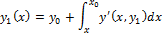
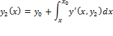
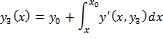
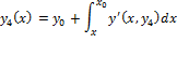
![]()
![]()
![]()
![]()
![]()
![]()
Predictor Formula ![]()
Corrector Formula ![]()
.
.
.
and so on till desired approximation is achieved
Adam Bashforth's Predictor formula ![]()
Adams Moulton's Corrector formula ![]()
It is a non-self-starting four step method which uses 4 initial
points ![]() to calculate
to calculate ![]() for
for ![]() . It requires only two function evaluation
of
. It requires only two function evaluation
of ![]() per step.
per step.

|
Circle
|
Ellipse
|
|
Segment of a line from point
|
|
![]()
![]()
![]()
· Line integral converted to double integral
![]()
· Line integral converted to surface integral and vice-versa
A vector field ![]() is called
conservative if a scalar function
is called
conservative if a scalar function ![]() can be found such
that
can be found such
that ![]() . The scalar function
. The scalar function
![]() is called potential
function of
is called potential
function of ![]() .
.
![]()
· Surface integral and Volume integral
|
Line integral w.r.t to arc
length |
|
|
Line integrals w.r.t variables |
|
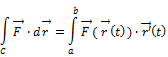
Given ![]() and
and ![]()
The line integral of
vector field ![]() is defined as
is defined as
A vector normal to
the curve ![]() is given by
is given by ![]()
·
![]() if
if ![]() where
where ![]() is a scalar function
is a scalar function
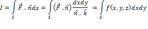
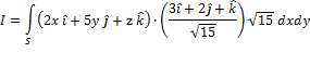
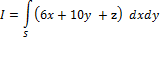
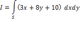
![]()
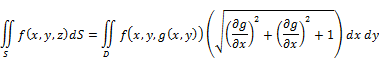
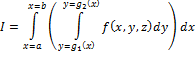
![]() where the surface S
is
where the surface S
is ![]() and D is the region
for double integration in the
and D is the region
for double integration in the ![]() plane.
plane.
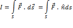
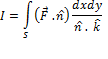
![]()
|
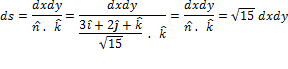
1.
Evaluate a unit normal vector
2.
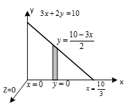
Projection* of
3.
Substitution for
4. After all the above substitution we have
5. Evaluate the multiple integral
|
Evaluate
1.
A vector normal to
2.
Projection of
3. After substitution
4. Substitute
5. Evaluate the double integral
|

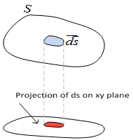


* The concept of projection of one vector over another is used here.
|
1. |
Abort execution of a command |
Alt+. |
|
2. |
Abort execution of a command |
Evaluation -> Quit Kernel -> Local |
|
3. |
Include a comment |
* Insert comments between asterisk * |
|
4. |
TraditionalForm[ |
|
|
5. |
Symbol=. |
Removes the value of the symbol |
|
6. |
Expression//Command |
It is the same as Command[Expression] |
|
7. |
N[Expression,n] |
attempts to give answer in n decimal digits |
|
8. |
?Command |
Gives help about the command |
|
9. |
??Command |
Gives help on the attributes and options of the command |
|
10. |
Ctrl+K |
Shows all command starting with say ‘Arc’ |
|
11. |
?Command* |
Shows all command beginning with say ‘Arc’ |
|
12. |
?`* |
Lists all global variables |
|
13. |
/. |
Replacement or Substitution |
|
14. |
/; |
Conditional |
|
15. |
Together[] |
Combines the difference or sum of fractions |
|
16. |
|
Function argument on the left hand side is always suffixed with an underscore in user defined functions |
|
17. |
:> or :-> |
Rule Delayed |
|
18 |
# & |
Pure function |
|
19. |
/@ |
Used to map a function to a list Map[f,list] f/@list |
Using: = is a must. The argument of the function is suffixed with an underscore.
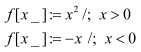
It is better to use Piecewise [ ] function to create such functions because limits and continuity can be then be checked.
Expression//MatrixForm
Expression//TableForm
Expression//TraditionalForm
|
NestList[] |
|
|
Range[] |
|
|
Array[] |
|
|
Table[] |
|
|
1. |
Solve [equation, variables] |
|
|
2. |
Reduce[equation, variables] |
|
|
3. |
Solve[equation, variables]//ComplexExpand |
Represents complex number in traditional form rather than as rational power |
|
4. |
Eliminate [equation, variables] |
Removes variable from a set of simultaneous equation |
|
5. |
NSolve [ equation, variables] |
Gives numerical solution |
|
6. |
FindRoot [equation, startingvalue] |
Gives solution to ‘transcendental equation’ |
|
7. |
LinearSolve [a,b] |
Produces
vector |
s=Solve[x^2+2x+1, x]
f[x]/.s
|
1. |
Together [] |
|
|
2. |
Apart [] |
|
|
3. |
Cancel [] |
|
|
UnitBox[x] |
Gives a rectangular pulse of width unity from -1/2 to 1/2 in the time domain |
|
|
Schaum's Vector Calculus(Spiegel) |